Wage Differences between three races

Introduction

This report explores the data set of roughly 25,000 records for males between the age of 18 and 70 who are full time workers and intend to answer the following two research questions with the final linear regression model that incorporates all relevant variables, interactions and functional forms of the covariates. The research questions are shown in the following paragraph:

1. Do African American males have statistically different wages compared to Caucasian males?
2. Do African American males have statistically different wages compared to all other males?

First, plot the scatter plots of different explanatory variables versus the explained variable, which is the logarithm of wage. The scatter plot of commuting distances versus log(wage) seems reasonable, forming a rectangular shape centering on a horizontal line.

Fig 1

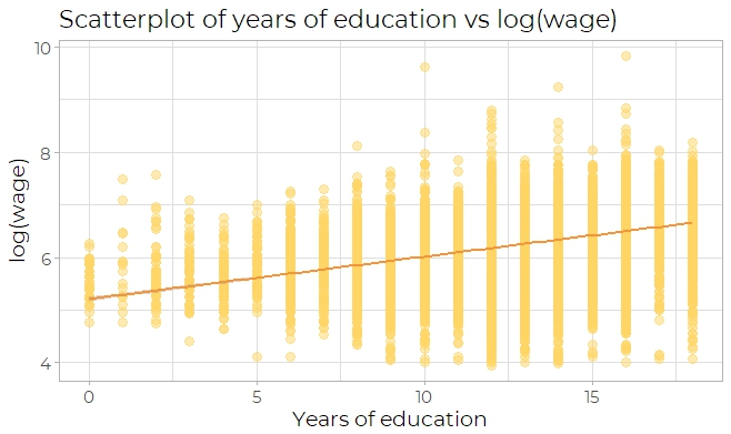
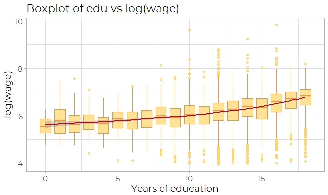
Then trying the scatter plot of years of education versus logarithm of wage, which has an increasing trend as years of education get larger (Fig 2a). This trend can be inspected more clearly by observing a box plot of education versus logarithm of wage(Fig 2b).

Fig 2a

Fig 2b

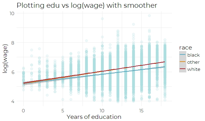
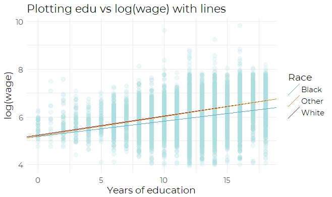
Next, it is suspected that race might have interactions with other explanatory variables. For example, we can try inspecting the interaction between race and education. By plotting the scatter plot of edu versus log(wage) and using the smoother(Fig 3a), we can observe that the African Americans get a lower wage compared to Caucasians and others. The same conclusion can be arrived by inspecting Fig 3b, the scatter plot of edu versus log(wage) using lines. Therefore, an interaction effect between education and race(the product of exp and race) is added to the refined model. After adding the interaction effect, run a R summary to check if the interaction is significant. Here is the interaction statistic taken from the summary output:

Coefficients:
                Estimate Std. Error t value Pr(>|t|)    
edu:raceother  1.744e-03  5.745e-03   0.304 0.761484    
edu:racewhite  4.590e-04  5.069e-03   0.091 0.927852     

It can be concluded that the interaction terms are not significant (p-values very large, bigger than 0.05). Therefore, it is safe to continue with this model.

Fig 3a

Fig 3b

In the above analysis, only the commuting distance and education scatterplots are checked, which is not enough for inspecting the model. Therefore, we plot the scatterplot relates to years of job experience (Fig 4) and the one for number of employees in a company (Fig 5). By inspecting the scatterplot of exp, it is obvious that it follows a curvilinear shape. Therefore, some adjustments should be made to the exp variable (i.e. adding a polynomial form of exp). The scatterplot of emp looks similar to the scatterplot of commuting distance. Therefore, no adjustment is needed for emp variable.

Fig 4

Fig 5

Statistical Model

The final model follows the following formula: $$log(wage) = edu + edu*race + exp + exp^2 + exp^3 + city + reg + race + deg + emp$$

Summary

Call:
lm(formula = log(wage) ~ edu + edu * race + exp + poly(exp, 3,
    raw = T) + city + reg + race + deg + emp, data = train.data)

Residuals:
    Min      1Q  Median      3Q     Max
-2.7969 -0.2915  0.0307  0.3293  3.9577

Coefficients: (1 not defined because of singularities)
                         Estimate Std. Error t value Pr(>|t|)    
(Intercept)             4.035e+00  6.328e-02  63.764  < 2e-16 ***
edu                     8.419e-02  4.774e-03  17.637  < 2e-16 ***
raceother               1.849e-01  7.122e-02   2.596 0.009436 **
racewhite               1.906e-01  6.207e-02   3.071 0.002140 **
exp                     8.633e-02  2.196e-03  39.309  < 2e-16 ***
poly(exp, 3, raw = T)1         NA         NA      NA       NA    
poly(exp, 3, raw = T)2 -2.482e-03  1.078e-04 -23.020  < 2e-16 ***
poly(exp, 3, raw = T)3  2.301e-05  1.501e-06  15.332  < 2e-16 ***
cityyes                 1.667e-01  8.465e-03  19.688  < 2e-16 ***
regnortheast            4.329e-02  1.071e-02   4.042 5.31e-05 ***
regsouth               -6.638e-02  9.944e-03  -6.675 2.54e-11 ***
regwest                -1.388e-02  1.082e-02  -1.283 0.199472    
degyes                  4.527e-02  1.205e-02   3.757 0.000172 ***
emp                     3.995e-04  4.918e-05   8.123 4.82e-16 ***
edu:raceother           4.556e-03  5.521e-03   0.825 0.409206    
edu:racewhite           4.388e-03  4.877e-03   0.900 0.368304    
---
Signif. codes:  0 ‘***’ 0.001 ‘**’ 0.01 ‘*’ 0.05 ‘.’ 0.1 ‘ ’ 1

Residual standard error: 0.5128 on 19843 degrees of freedom
Multiple R-squared:  0.3486,	Adjusted R-squared:  0.3482
F-statistic: 758.6 on 14 and 19843 DF,  p-value: < 2.2e-16

The model included an interaction between edu and race, a logarithm transformation of wage and a polynomial form of exp (exp, exp^2 and exp^3). The R^2 is 0.3486. The adjusted R^2 is 0.3482. The AIC is 29843.85.

Research Question

Question 1

• Step 1) State null hypothesis and alternative hypothesis
  H0: race black=race white
  HA: race black ≠ race white
• Step 2) Check the value of p-value Look at the summary output, the p-value of racewhite is 0.002140, which is lower than 0.05. Therefore, we reject the null hypothesis that the African American males have the same wages as Caucasian males. So African American males have statistically different wages compared to Caucasian males.

Question 2

• Step 1) State the null hypothesis and alternative hypothesis
  H0: race black = race white = race other
  HA: race black ≠ at least one race
• Step 2) Check the value of p-value

Analysis of Variance Table

Response: log(wage)
                         Df Sum Sq Mean Sq   F value    Pr(>F)    
edu                       1 1094.9 1094.90 4164.2243 < 2.2e-16 ***
race                      2   88.9   44.43  168.9733 < 2.2e-16 ***
exp                       1  977.2  977.22 3716.6565 < 2.2e-16 ***
poly(exp, 3, raw = T)     2  459.8  229.88  874.2892 < 2.2e-16 ***
city                      1  118.9  118.90  452.2288 < 2.2e-16 ***
reg                       3   31.5   10.49   39.8780 < 2.2e-16 ***
deg                       1    3.8    3.83   14.5490  0.000137 ***
emp                       1   17.3   17.32   65.8619 5.116e-16 ***
edu:race                  2    0.2    0.11    0.4191  0.657622    
Residuals             19843 5217.3    0.26                        
---
Signif. codes:  0 ‘***’ 0.001 ‘**’ 0.01 ‘*’ 0.05 ‘.’ 0.1 ‘ ’ 1

The p-value of race is less than 2.2e-16, which is much lower than 0.05. Therefore, we reject the null hypothesis that African American males have the same wages as all other males. So African American males have statistically different wages compared to all other males.

Appendix

a. Model Selection

In this model, a logarithm transformation is applied to the response variable (wage). By inspecting the qq plot (Fig 6a), it is clear that the right tail of the shape departs from linearity, which suggests that the error distribution is not normal. Therefore, a logarithm transformation of wage should be performed. After adjusting the model, the qq plot (Fig 6b) seems more linear than before.

Fig 6a

Fig 6b

An interaction between edu and race is used in model. This is because the scatter plot (Fig 3a and Fig 3b) shows a relationship between edu and race: as years of education increases, log(wage) also increases; however, black people keep having a wage lower than other races. Therefore, this interaction is included. After adding the interaction term, a best subset algorithm is used based on AIC. The output is showed in the following paragraph:

AIC
Best Model:
               Df Sum Sq Mean Sq  F value  Pr(>F)    
data.edu        1   1095  1094.9 3820.537 < 2e-16 ***
data.exp        1    981   981.0 3423.246 < 2e-16 ***
data.city       1     99    99.2  346.206 < 2e-16 ***
data.reg        3     46    15.3   53.219 < 2e-16 ***
data.race       2     79    39.5  137.715 < 2e-16 ***
data.deg        1      2     2.2    7.721 0.00546 **
data.emp        1     20    19.9   69.464 < 2e-16 ***
Residuals   19847   5688     0.3                     
---
Signif. codes:  0 ‘***’ 0.001 ‘**’ 0.01 ‘*’ 0.05 ‘.’ 0.1 ‘ ’ 1

This output suggests that we should drop the com variable. After dropping the unnecessary variable, we go back to the EDA process and plot the scatter plots of exp versus log(wage) (Fig 4) and emp versus log(wage) (Fig 5), which by inspecting those plots, it can be recognized that the exp variable exhibits a curvilinear form, and therefore can be expressed in a polynomial functional form. We first tried to add exp^2, but resulted in significant interaction term: edu:racewhite with p-value of 0.033508. Therefore, exp^3 is tried and resulted in insignificant interaction terms.

              p-value
edu:raceother 0.409206
edu:racewhite 0.368304

b. Diagnostics and Model Validation

There are four kinds of plots used in this diagnostic process: qq plot, residual plot, box plot and line plot. The first one used is the qq plot (Fig 7), which looks like the qq plot after the log transformation and the linearity is acceptable.

Fig 7

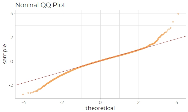
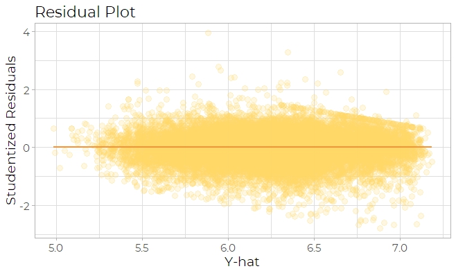
The second kind of diagnostic plot used is residual plot, which can be categorized into two section: one is fitted y value versus Studentized residuals, and the other is explanatory variable versus Studentized residuals. The residual plot of y hat versus Studentized residuals (Fig 8a) seems appropriate because the residuals fall within a horizontal band centered around 0.

Fig 8a

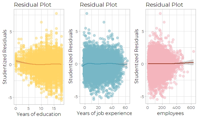
By inspecting the three scatter plots of explanatory variables versus Studentized residuals (Fig 8b), it can be seen that the shape of residuals are in good shape: centered around 0 in a horizontal fashion.

Fig 8b

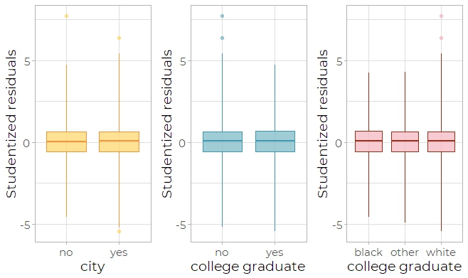
The third diagnostic plot is the box plot (Fig 9), which plots the categorical variables versus the Studentized residuals. Only a few outliers exist, which means this model is appropriate in normality.

Fig 9

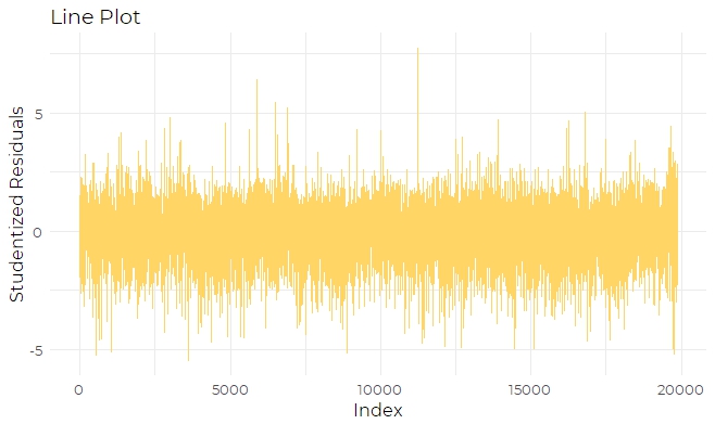
The final diagnostic plot is the line plot (Fig 10), which detects whether there are dependent errors in the model. The line plot does not exhibit any pattern, so it indicates that this model has independent errors, which is appropriate.

Fig 10

The MSE of the final model is 0.26, and the computed MSPR is 0.263, which is fairly close to MSE, a good indication of the predictive ability of the model.