Introduction
As for application of this model in real life problem, we decide to study fuel consumption for cars. Nowadays, petroleum consumption of cars is an important question that we pay attention to. In this case, we decide to study the “mtcars” dataset in R that contains some information about fuel consumption and its affected factors. Particularly, we are interested how gross horse power and rear axle ratio affect the miles per gallon for cars.
Hierarchical Linear regression
Usually, the hierarchical linear regression contains a 2-level structure, which is also we adopt in this project. Further levels could be considered but not very practical. The inclusion of higher than 2 levels in the hierarchical linear regression is similar to that of making assumptions on prior distributions of the hyper-parameters in the Bayesian context. In the 2-level case, we specify the individual-specific regression coefficients with a joint distribution at level 2. A comparison among different models: no pooling(separate regression without grouping), complete pooling(putting all in one group) and hierarchical(idea of partial pooling, sharing the advantage of both) shows that inappropriate grouping could yield completely opposite result from the truth.
Application using RStan
This classification of different quantities into blocks in effect strengthened our understanding of the structure of the model in a comprehensive way. The details of our use of RStan to build the model will be unfolded in the following sections explaining our case of regression model.
Mathematical Background
= dependent variable
= intercept for level-2 unit
= regression coefficient vector associated with X for level-2 unit
r = random error vector associated with level-1 unit nested within the level-2 unit
E(r) = 0; var(r) =
Model Analysis
Step 0. Data and parameters preparation
library(rstan)
setwd("C:/Users/SHE3/Desktop/Data")
> fit <- lm(mpg~hp+drat,data=mtcars)
> fit

Call:
lm(formula = mpg ~ hp + drat, data = mtcars)

Coefficients:
(Intercept)           hp         drat
   10.78986     -0.05179      4.69816

> summary(fit)

Call:
lm(formula = mpg ~ hp + drat, data = mtcars)

Residuals:
    Min      1Q  Median      3Q     Max
-5.0369 -2.3487 -0.6034  1.1897  7.7500

Coefficients:
             Estimate Std. Error t value Pr(>|t|)
(Intercept) 10.789861   5.077752   2.125 0.042238 *
hp          -0.051787   0.009293  -5.573 5.17e-06 ***
drat         4.698158   1.191633   3.943 0.000467 ***
---
Signif. codes:  0 ‘***’ 0.001 ‘**’ 0.01 ‘*’ 0.05 ‘.’ 0.1 ‘ ’ 1

Residual standard error: 3.17 on 29 degrees of freedom
Multiple R-squared:  0.7412,	Adjusted R-squared:  0.7233
F-statistic: 41.52 on 2 and 29 DF,  p-value: 3.081e-09
> sd(mtcars$mpg)
[1] 6.026948
#simulate some data
set.seed(20180417)
N<-500 #sample size
J<-10 #number of car types
id<-rep(1:J,each=50) #index of car types
K<-3 #number of regression coefficients
#population-level regression coefficient
gamma<-c(10,-0.05,5)
#standard deviation of the group-level coefficient
tau<-c(5,0.1,1)
#standard deviation of individual observations
sigma<-6
#group-level regression coefficients
beta<-mapply(function(g,t) rnorm(J,g,t),g=gamma,t=tau)
#the model matrix
X<-model.matrix(~x+y,data=data.frame(x=runif(N,-2,2),y=runif(N,-2,2)))
y<-vector(length = N)
for(n in 1:N){
  #simulate response data
  y[n]<-rnorm(1,X[n,]%*%beta[id[n],],sigma)
}
Step 1. Specify likelihood and prior distributions
data {
    int<lower=1> N; //the number of observations
    int<lower=1> J; //the number of groups
    int<lower=1> K; //number of columns in the model matrix
    int<lower=1,upper=J> id[N]; //vector of group indices
    matrix[N,K] X; //the model matrix
    vector[N] y; //the response variable
  }
parameters {
  vector[K] gamma; //population-level regression coefficients
  vector<lower=0>[K] tau; //the standard deviation of the regression coefficients
  vector[K] beta_raw[J];
  real<lower=0> sigma; //standard deviation of the individual observations
}
transformed parameters {
  vector[K] beta[J]; //matrix of group-level regression coefficients
  //computing the group-level coefficient, based on non-centered parameterization based on section 22.6 STAN (v2.12) user's guide
  for(j in 1:J){
    beta[j] = gamma + tau .* beta_raw[j];
  }
}
model {
  vector[N] mu; //linear predictor
  //priors
  gamma ~ normal(0,5); //weakly informative priors on the regression coefficients
  tau ~ cauchy(0,2.5); //weakly informative priors, see section 6.9 in STAN user guide
  sigma ~ gamma(2,0.1); //weakly informative priors, see section 6.9 in STAN user guide
  for(j in 1:J){
   beta_raw[j] ~ normal(0,1); //fill the matrix of group-level regression coefficients;
   //implies beta~normal(gamma,tau)
  }
  for(n in 1:N){
    mu[n] = X[n] * beta[id[n]]; //compute the linear predictor using relevant group-level regression coefficients
  }
  //likelihood
  y ~ normal(mu,sigma);
}
We chose three weakly informative priors for our parameters, which are normal(0, 5) for gamma (the population level regression coefficients), cauchy(0, 2.5) for tau (the standard deviation of the regression coefficients) and gamma(2,0.1) for sigma (standard deviation of the individual observation). The weakly informative priors are useful because they provide some information on the relative a priori plausibility of the possible parameter values. They also help to reduce posterior uncertainty and stabilize computations.
Step 2. Estimate model parameters
m_hier<-stan(file="newmodel.stan",data=list(N=N,J=J,K=K,id=id,X=X,y=y))
Inference for Stan model: newmodel.
4 chains, each with iter=2000; warmup=1000; thin=1;
post-warmup draws per chain=1000, total post-warmup draws=4000.

          mean se_mean   sd  2.5%   25%   50%  75% 97.5% n_eff Rhat
gamma[1]  8.96    0.04 1.22  6.30  8.23  9.02 9.77 11.21  1097    1
gamma[2] -0.14    0.00 0.28 -0.69 -0.32 -0.14 0.04  0.43  3454    1
gamma[3]  4.95    0.01 0.36  4.22  4.73  4.95 5.18  5.64  2188    1
tau[1]    3.55    0.03 0.99  2.14  2.84  3.38 4.05  5.98  1299    1
tau[2]    0.34    0.01 0.28  0.01  0.13  0.29 0.49  1.02  1906    1
tau[3]    0.71    0.01 0.43  0.06  0.41  0.67 0.95  1.64  1445    1
sigma     6.05    0.00 0.19  5.69  5.92  6.05 6.19  6.43  4000    1

Samples were drawn using NUTS(diag_e) at Sat Apr 21 18:08:57 2018.
For each parameter, n_eff is a crude measure of effective sample size,
and Rhat is the potential scale reduction factor on split chains (at
convergence, Rhat=1).
Step 3. Check sampling quality
> library(shinystan)
> launch_shinystan(m_hier)


Step 4. Summarize and interpret results
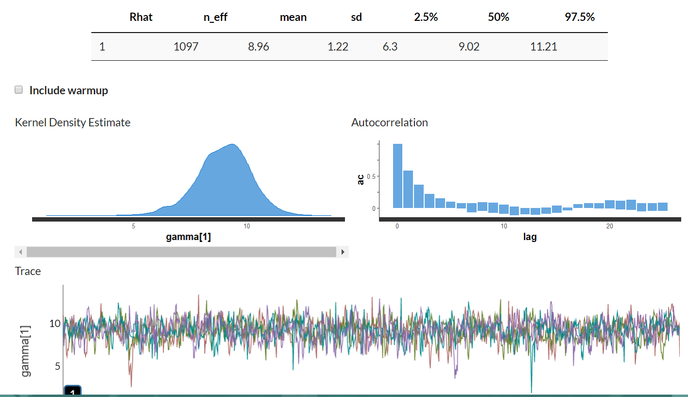
A measure of central tendency (mean, median) that chosen to summarize a posterior distribution is a point estimate, which is a single value. In the Bayesian framework, we are interested in the entire posterior distribution rather than the point estimate.

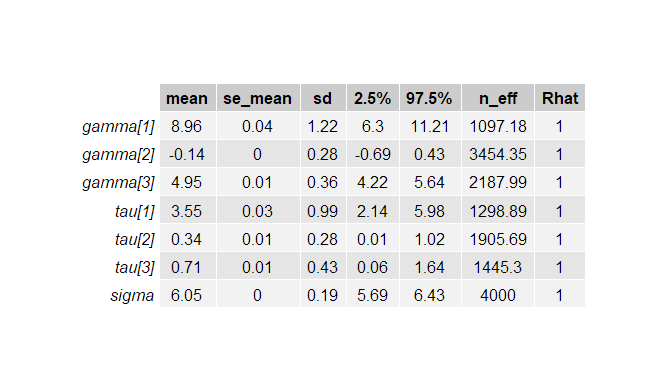
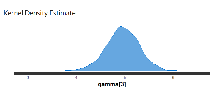
From observing Table 1, the point estimate (in this case which is the mean of the posterior distribution) for the gamma 1 is 8.96, with 95% PI=[6.3,11.21]. The estimate for the population level regression coefficient gamma 3 (which corresponds to rear axle ratio) indicates that a one unit change in rear axle ratio is associated with an increase of 4.95 (95%PI = [4.22,5.64]) in mpg (miles per gallon) value. In Figure 3, the posterior probability distribution plot of the regression coefficient shows that the probability mass for this parameter is on positive values, suggesting that mpg value is remarkably associated with rear axle ratio.

Conclusion
Discussion
Particularly, the philosophical concept of compromising between models came into view, though only in a general and inconspicuous way, and for the time being not showing direct helpfulness to applications. For example, the analogy of bayesian philosophy (balancing between prior belief and real data for the estimation of model parameters) and hierarchical models (in the sense of compromising between aggregate and disaggregate models) even in the context of regression has broadened our horizon.
Meanwhile, the smooth implementation and compact representation of the model in RStan demonstrated itself bunches of its advantages such as scalability, efficiency and robustness. Its clear-cut structure also aroused our interest in other possible extensions which have not been carried out in it such as user specific functions and non-conjugate prior, which could be another direction of future research.
Appendix
Contribution Statement
Dataset
> mtcars
                     mpg cyl  disp  hp drat    wt  qsec vs am gear carb
Mazda RX4           21.0   6 160.0 110 3.90 2.620 16.46  0  1    4    4
Mazda RX4 Wag       21.0   6 160.0 110 3.90 2.875 17.02  0  1    4    4
Datsun 710          22.8   4 108.0  93 3.85 2.320 18.61  1  1    4    1
Hornet 4 Drive      21.4   6 258.0 110 3.08 3.215 19.44  1  0    3    1
Hornet Sportabout   18.7   8 360.0 175 3.15 3.440 17.02  0  0    3    2
Valiant             18.1   6 225.0 105 2.76 3.460 20.22  1  0    3    1
Duster 360          14.3   8 360.0 245 3.21 3.570 15.84  0  0    3    4
Merc 240D           24.4   4 146.7  62 3.69 3.190 20.00  1  0    4    2
Merc 230            22.8   4 140.8  95 3.92 3.150 22.90  1  0    4    2
Merc 280            19.2   6 167.6 123 3.92 3.440 18.30  1  0    4    4
Merc 280C           17.8   6 167.6 123 3.92 3.440 18.90  1  0    4    4
Merc 450SE          16.4   8 275.8 180 3.07 4.070 17.40  0  0    3    3
Merc 450SL          17.3   8 275.8 180 3.07 3.730 17.60  0  0    3    3
Merc 450SLC         15.2   8 275.8 180 3.07 3.780 18.00  0  0    3    3
Cadillac Fleetwood  10.4   8 472.0 205 2.93 5.250 17.98  0  0    3    4
Lincoln Continental 10.4   8 460.0 215 3.00 5.424 17.82  0  0    3    4
Chrysler Imperial   14.7   8 440.0 230 3.23 5.345 17.42  0  0    3    4
Fiat 128            32.4   4  78.7  66 4.08 2.200 19.47  1  1    4    1
Honda Civic         30.4   4  75.7  52 4.93 1.615 18.52  1  1    4    2
Toyota Corolla      33.9   4  71.1  65 4.22 1.835 19.90  1  1    4    1
Toyota Corona       21.5   4 120.1  97 3.70 2.465 20.01  1  0    3    1
Dodge Challenger    15.5   8 318.0 150 2.76 3.520 16.87  0  0    3    2
AMC Javelin         15.2   8 304.0 150 3.15 3.435 17.30  0  0    3    2
Camaro Z28          13.3   8 350.0 245 3.73 3.840 15.41  0  0    3    4
Pontiac Firebird    19.2   8 400.0 175 3.08 3.845 17.05  0  0    3    2
Fiat X1-9           27.3   4  79.0  66 4.08 1.935 18.90  1  1    4    1
Porsche 914-2       26.0   4 120.3  91 4.43 2.140 16.70  0  1    5    2
Lotus Europa        30.4   4  95.1 113 3.77 1.513 16.90  1  1    5    2
Ford Pantera L      15.8   8 351.0 264 4.22 3.170 14.50  0  1    5    4
Ferrari Dino        19.7   6 145.0 175 3.62 2.770 15.50  0  1    5    6
Maserati Bora       15.0   8 301.0 335 3.54 3.570 14.60  0  1    5    8
Volvo 142E          21.4   4 121.0 109 4.11 2.780 18.60  1  1    4    2
Reference
- Muth, Chelsea, et al. “User-Friendly Bayesian Regression Modeling: A Tutorial with Rstanarm and Shinystan.” The Quantitative Methods for Psychology, vol. 14, no. 2, Jan. 2018, pp. 99–119., doi:10.20982/tqmp.14.2.p099.
- biologyforfun
- datascienceplus
- Stan_lectures
- The quantitative methods for Psychology
