Summary
Here is the url for the code.
This report presents an analysis for the recent 5 years data of 10 companies, Apple, Amazon, Bank of America, Facebook, Google, IBM, JP Morgan, Microsoft, Target and Walmart. Also, Monthly closing price from November 11, 2013 to November 11, 2018 are used to compute monthly returns of each company for the further analysis. The report contains 5 statistical analysis parts separated by the topics and a data description part. Main results are shown below:
This report presents an analysis for the recent 5 years data of 10 companies, Apple, Amazon, Bank of America, Facebook, Google, IBM, JP Morgan, Microsoft, Target and Walmart. Also, Monthly closing price from November 11, 2013 to November 11, 2018 are used to compute monthly returns of each company for the further analysis. The report contains 5 statistical analysis parts separated by the topics and a data description part. Main results are shown below:
- Overall, due to the stock market selloff during 2015-2016, all the stocks did not perform well in 2015 and 2016. In addition, among these ten stocks, there are three stocks, Apple, Facebook, and Target are seemly normally distributed, and Amazon is the most risky stock.
- Microsoft and Amazon are most highly correlated with the value of 0.983 while Facebook and IBM are least correlated with the value of -0.577. The diversification will benefit more when the assets have a lower correlation value. Principal component analysis demonstrates that the first three components can represent the distribution of data and variation of the stock price, explaining 93.5% of the variance of data.
- Among the 4 copulas(normal, t, Clayton, Gumbel), t copula fits the data best since it has the smallest AIC value. Normal copula is similar to t copula and performs relatively well also because the estimate v of t copula is large.
- the minimum variance portfolio of 10 assets has monthly mean of 0.00918 and standard deviation of 0.00084, with the weight of 0.060,-0.080,-0.176,0.169,0.173,0.100,0.454,-0.011,0.047 and 0.265 respectively(alphabetical order). Each individual assets has a sharp ratio under 1. Therefore, a tangency portfolio is constructed with a sharpe ratio of 0.376, better than the individual asset.
- An efficient portfolio which can achieve 6% expected return per year with only risky assets and no short sales consists 9.5% of Facebook, 7.4% of Google, 31.2% of IBM, 10.1% of JP Morgan, 9.3 of Target and 32.5% of Walmart. Combining the efficient portfolio with other conditions remaining the same, a new portfolio is created consisting of 92.3% of T-bills, 2.4% of Facebook, 0.5% of Apple, 1.5% of Amazon, 1.7% of JP Morgan, 1.5% of Microsoft and 0.1% of Walmart. The 5% value at risk for both portfolios are the same because T-bills are risk free and hence will not cause any loss in the extreme event.
- There are two ways to estimate 5% value at risk(VaR) and expected shortfall(ES). For the parametric method, Amazon has the highest 5% VaR and ES, while JP Morgan has the lowest value for both. For the nonparametric method, Bank of America has the highest VaR and Google has the lowest. Also, IBM has the highest ES and Google has the lowest ES.
Descriptive Statistics
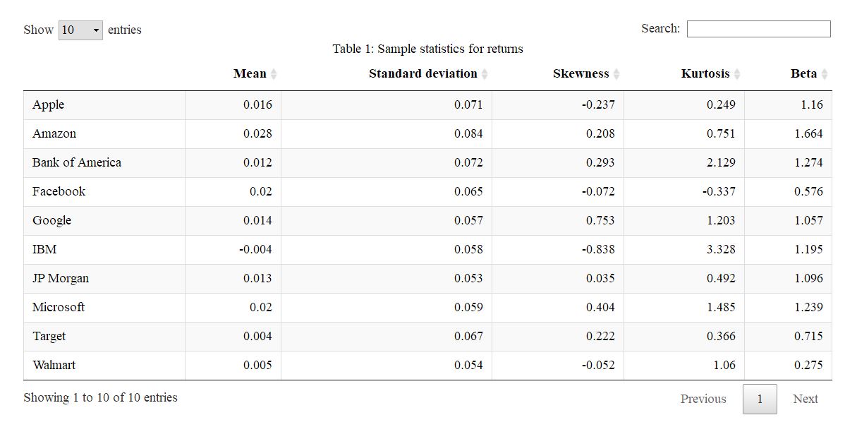 We have chosen ten assets and computed the sample statistics for monthly returns based on a five year
period(2013/11 to 2018/11). From the sample statistics table for returns, it can be seen that IBM has a
negative average of returns. The firm does not perform very well since 2016, which can be verified on the
monthly price and return plot and also on the news. Part of the reasons can be that IBM is shifting away
from its legacy software business towards cloud computing.
When checking the standard deviation (risk) , it is obvious that Amazon has the highest risk. One reason that Amazon possess a great risk may be due to the fierce competition it is facing: there are Best Buy, Walmart and Target that also sell online merchandise.
From the skewness coefficient column, it can be seen that both IBM and Google are moderately skewed: it can be verified in the histogram plot where Google skewed to right and IBM skewed to left(Fig 2(c)). Compared to skewness, the kurtosis coefficient is more diverse, ranging from -0.337 to 3.328. The distributions that perform most close to Normal distributions are the ones of IBM and Bank of America, with a kurtosis coefficient of 3.328 and 2.129. The last sample statistic is beta, and a large amount of the stocks are aggressive and risky. Amazon has the highest beta here, bearing a higher systematic risk than others. In contrast, one of Amazon’s opponents, Walmart has the lowest beta, which indicates it is not aggressive compared to others.
When inspecting plots of monthly price and returns, it can be seen that it was a hard time for the companies from 2015 to 2016(Fig 1). This is because the 2015-2016 stock market selloff , which was the period of decline of the value of stock prices globally. A series of events occured that time to cause investors sold shares globally: first the slowing growth of GDP in China, the decline in petroleum prices, the Greek debt default happened in June 2015, the effects of the end of quantitative easing in the United States and finally the United Kingdom European Union membership referendum (Brexit). There are also some unusual outliers for the returns. For example, in 2015 July(Fig 1(e)), Google’s return increased dramatically. The number increased right after Google reported its second quarter earnings, which rose 11% year to year to $17.7 billion that time.
Apart from monthly return plots, there are also histograms, box plots and qq plots that worth examining. First, when looking at histograms, we can see that some look like normally distributed, some are skewed and some are not unimodal distributed. We have verified the skewness of IBM and Google by both examining the skewness coefficients and looking at the density of histograms(Fig 2(c)). It is also worth noticing that Microsoft has a kurtosis coefficient of 1.485, which indicates a peaked distribution and can also be verified in the density histogram(Fig 2(d)).
Secondly, when looking at boxplots(Fig 3), we can see that roughly all the returns have a similar median, but with some unusually tall boxes and compact boxes. The Amazon stock has the tallest box, which again proves it has a high standard deviation(risk). On the other hand, JP Morgan has the most compact box, with the lowest standard deviation. Some of the stocks look normally distributed according to box plot (evenly proportioned box and same length whiskers): Apple, Facebook, Google and Target.
Let’s move to the qq plot to check if they are actually normal: the plots for Apple, Facebook and Target looks very normal, which means the dots can fit onto a line(Fig 4). However, Google’s plot seems a bit heavy tailed(Fig 4(c)). By looking at the three plots, I came to conclusion that Apple, Facebook and Target’s distributions are seemingly normally distributed.
The next step in the descriptive statistics is to construct pairwise scatter plots(Fig 5) and observe the relationships between stocks. It is worth noting that Bank of America and JP Morgan seem positively correlated(with a correlation coefficient of 0.875). This can be understandable because they are both in the banking industry. Besides this pair, Google and Amazon also seems positively correlated(with a correlation coefficient of 0.626). This is because they are both high technology firms.
In conclusion, there are three seemingly normally distributed stocks: Apple, Facebook and Target. Also, Amazon is the most risky stock among these 10 stocks. Finally, those 10 stocks did not perform well from 2015 to 2016 because of the 2015-2016 stock market selloff.
Principal Component Analysis
In this section, we conduct factor analysis and principal component analysis for the following ten assets’
monthly closing prices from 11/1/2013 to 11/1/2018: AAPL, AMZN, BAC, FB, GOOG, IBM, JPM,
MSFT, TGT, WMT. Since there exists high degree of collinearity between these stocks’ returns, it is
difficult to visualize and analyze this ten-dimensional data in our datasets. Thus, it is helpful to use
dimension reduction to extract important sources of information in the data. The idea of principal
component analysis is to find structure in the correlation matrix and use this structure to locate
low-dimensional subspaces containing most of the variation in the data.
First, we computed the sample correlation matrix of the returns on ten assets. The result shows that Microsoft and Amazon are most highly correlated with correlation of 0.9831232, while Facebook and IBM are least correlated with correlation of -0.5771376. Diversification will reduce risk with these assets based on the estimated correlation values. The less correlated assets are, the more gain from diversification.
Next, we run the principal component analysis and found 10 principal components. The first principal component is a linear combination of -0.352 Apple return, -0.362 Amazon return, -0.348 Bank of America return, -0.341 Facebook return, -0.36 Google return, 0.212 IBM return, -0.362 JP Morgan return, -0.367 Microsoft return, -0.25 Walmart return. Amazon, Microsoft, Google and JP Morgan are all very significant in the first component, which means that these stocks prices vary a lot compared to others. The second principal component which is orthogonal to the first principal component is a linear combination of -0.226 Bank of America return, -0.569 IBM return, -0.13 JP Morgan return, 0.735 Target return, -0.249 Walmart return. Both the first and second principal components can explain the variance in Bank of America, IBM, JP Morgan, Target and Walmart.
The proportion of variance for each principal component can explain the amount of information gain. The summary of principal component analysis shows that first principal component can explain 72.5% of the variance of our data, the second principal component can explain 13.1% of the variance of the data, the third principal component can explain 7.9% of the variance of the data. Thus, the first three components can represent the distribution of the data and variation of the stocks prices.
Copulas
We use 4 copulas, normal, t, Clayton and Gumbel, to model the joint distribution of the 10 companies’
returns. Due to the two potential problems with the maximum likelihood estimation, we apply the
semiparametric approach to pseudo-maximum likelihood estimation, estimating the distribution of each
return nonparametrically and estimating the copula parametrically.
First, to estimate the distribution non parametrically, we rank each company’s return and divide by n+1, n is the sample size. Then, for the second step of the pseudo-maximum likelihood method, since the data includes 10 companies, it has relatively high dimensions with 10*9/2 = 45 correlation parameters. This high dimensions may cause difficulties in maximization, Therefore when fitting the normal and t copulas, we compute the Spearman rank correlation first and then choose a starting value in order to reduce the difficulties. Finally, after modeling the joint distribution of the returns, AIC values are computed to determine which copula fits the data best. Following are the results:
From the AIC values shown above, we can conclude that t copula fits the data best because it has the smallest value. Also, the normal copula fits relatively well and it is similar to the t copula since v = 22.204 is large. This conclusion is reasonable because Archimedean copulas are more useful in a bivariate case or in a multivariate case with all the pairs have similar dependencies.
First, to estimate the distribution non parametrically, we rank each company’s return and divide by n+1, n is the sample size. Then, for the second step of the pseudo-maximum likelihood method, since the data includes 10 companies, it has relatively high dimensions with 10*9/2 = 45 correlation parameters. This high dimensions may cause difficulties in maximization, Therefore when fitting the normal and t copulas, we compute the Spearman rank correlation first and then choose a starting value in order to reduce the difficulties. Finally, after modeling the joint distribution of the returns, AIC values are computed to determine which copula fits the data best. Following are the results:
| Copula family | Estimates | Maximized log-likelihood | AIC |
|---|---|---|---|
| Normal | ρ = 0.8890085 | 1097 | -2192.34 |
| t | ρ = 0.8935737,v = 22.2041449 | 1103 | -2202.767 |
| Clayton | θ = 1.138399 | 960.1 | -1918.196 |
| Gumbel | θ = 4.515913 | 1066 | -2130.852 |
From the AIC values shown above, we can conclude that t copula fits the data best because it has the smallest value. Also, the normal copula fits relatively well and it is similar to the t copula since v = 22.204 is large. This conclusion is reasonable because Archimedean copulas are more useful in a bivariate case or in a multivariate case with all the pairs have similar dependencies.
Portfolio Theory
The portfolio includes all of the 10 assets and the minimum variance portfolio is constructed. The mean
and standard deviation (monthly) of the minimum variance portfolio is 0.00918 and 0.00084. The weights
of this portfolio are 0.060,-0.080,-0.176,0.169,0.173,0.100,0.454,-0.011,0.047 and 0.265. We can see that
we short saled 3 assets, which are Amazon, Bank of America and Microsoft. And this means that the
money get from shorting these assets is invested in other assets. Also, it is obvious that JP Morgan
occupied the most weight in the portfolio.
Assume that there is $100,000 to invest, the 5% value at risk for the minimum variance portfolio is approximately -$780. The 5% value at risk for the individual assets is very different: ranges from -$10470 to -$6258. VaR represents the maximal probable loss for a portfolio over a specified trading horizon and stated probability level. It is obvious that the minimum variance portfolio will incur the minimum loss of money while the individual assets will incur a much greater loss.
Aside from VaR, Sharpe Ratio is also an important measure to examine the performance of an investment by adjusting for its risk. It is worth noting that IBM has a negative Sharpe ratio, which is due to its negative return. By examining the Sharpe ratio of individual assets, we can see that they are all under 1, which is not very acceptable. After that, we constructed tangency portfolio using the risk free rate and ended up with a 0.376 Sharpe ratio, which is slightly better than the ones of individual assets.
Asset Allocation
In order to achieve a 6% annually target expected return using only risky assets, we need to construct an
efficient portfolio with our ten stocks to earn a 0.5% expected return monthly. Under the no short selling
constraint, the efficient portfolio consists of 9.5% of Facebook, 7.4% of Google, 31.2% of IBM, 10.1% of
JP Morgan, 9.3% of Target and 32.5% of Walmart. Other stocks have weight of 0 in the efficient
portfolio. The standard deviation is 0.0328, which is the monthly risk of this portfolio. If we invest
$100,000 initially, we should provide $9,486.5 capital for Facebook, $7,448.5 for Google, $31,174.2 for
IBM, $10,068 for JP Morgan, $9,310.9 for Target, and $32,511.9 for Walmart. The monthly 5%
value-at-risk is $362.24 which means there is 5% chance that our portfolio will lose at least $362.24 in a
month.
If we could add risk free asset, which is T-bills in the portfolio to achieve the same expected return, 6% per year or 0.5% per month, we need to find the tangency portfolio first, which gives the highest Sharpe ratio among all possible portfolios consisting of the ten risky stocks. Then T-bills are added to construct our portfolio, which accounts 92.3% of the total investment. Among ten stocks, Facebook weighs the most, which is 2.4%; other stocks we would invest in are Apple, Amazon, JP Morgan, Microsoft and Walmart, each has weight of 0.5%, 1.5%, 1.7%, 1.5%, and 0.1% respectively. Similarly, if the total investment is $100,000, we would invest $529.7 in Apple, $1,520.8 in Amazon, $2,380.8 in Facebook, $1,660.4 in JP Morgan, $1,520.1 in Microsoft, $123 in Walmart and $92,265.3 in T-bills. Since T-bills are risk free, the risk of the portfolio comes from risk assets only, which is 0.0032. This is the monthly standard deviation. Similarly, the 5% monthly value-at-risk is also $362.24.
This value is same for the efficient portfolio we constructed using risky assets only. This is because T-bills are risk free which will not cause any lost in the extreme event and we are using exactly same ten risky assets to construct a portfolio to achieve the same expected return. Therefore, under the worse circumstances, the portfolio contains T-bills will has same value-at-risk as the efficient portfolio before.
Risk Management
Risk management for financial market is very important. we will use value of risk and expected shortfall
as the risk metrics. Value at risk can measure the magnitude of extreme event, while expected shortfall
can measure the average loss of extreme event.
Assume we have 100,000 dollars to invest, we used parametric method and bootstrap to compute value at risk and expected shortfall for each of the ten assets in our portfolio. The results show that Amazon has the highest 5% value at risk, which means there is 5% chance of a loss exceeding 10816.222 dollars over one month. We are 95% confident that the 5% value at risk for Amazon is between 9153.901 dollars and 12478.542 dollars. JP Morgan has the lowest 5% value at risk, so there is 5% chance of a loss exceeding 7452.009 dollars over a month. We are 95% confident that the 5% value at risk for JP Morgan is between 6334.754 dollars and 8569.265 dollars. Amazon also has the highest expected shortfall, so we expect to loss 14271.299 dollars on average over a month. We are 95% confident that the expected shortfall for Amazon is between 12300.118 dollars and 16242.48 dollars. JP Morgan has the lowest expected shortfall, so we expect to loss 9660.689 dollars on average over a month. We are 95% confident that the 5% expected shortfall for JP Morgan is between 8354.649 dollars and 10966.73 dollars.
In addition, we used nonparametric method and bootstrap to compute value at risk and expected shortfall for each of the ten assets in our portfolio. The results show that Bank of America has the highest 5% value at risk, which means there is 5% chance of a loss exceeding 10813.881 dollars over one month. We are 95% confident that the 5% value at risk for Bank of America is between 8215.450 dollars and 13412.312 dollars. Google has the lowest 5% value at risk, so there is 5% chance of a loss exceeding 6621.631 dollars over a month. We are 95% confident that the 5% value at risk for Google is between 5750.489 dollars and 7492.774 dollars. IBM has the highest expected shortfall, so we expect to loss 15618.524 dollars on average over a month. We are 95% confident that the expected shortfall for IBM is between 9856.573 dollars and 21380.475 dollars. Google has the lowest expected shortfall, so we expect to lose 8038.984 dollars on average over a month. We are 95% confident that the expected shortfall for Google is between 6333.726 dollars and 9744.242 dollars.
Conclusion
We start to calculate the returns with most recent 5 years monthly closing price of 10 well-known
companies, Apple, Amazon, Bank of America, Facebook, Google, IBM, JP Morgan, Microsoft, Target
and Walmart. Then we conduct exploratory data analysis as the elementary step to study the data. The
very first thing we notice is that all stocks performed bearish during 2015-2016 because of the stock
market selloff and Amazon appears to be the most riskiest one.
Next, we use principal component analysis on the data and find out that Microsoft and Amazon are most highly correlated with the correlation of 0.983 while Facebook and IBM are least correlated with the correlation of -0.577. In total, the first three components can explain 93.5% of the variance of the data. Under the AIC criteria, t copula fits the data best. Since the estimate v of t copula is large enough, normal copula also performs very well.
After the analysis of correlation and distribution of the returns, we are able to find the minimum variance portfolio of these ten stocks. The monthly expected return is 0.9% and the risk is 0.00084. Each stock has a weight of 0.060, -0.080,-0.176,0.169,0.173,0.100,0.454,-0.011,0.047 and 0.265 for Apple, Amazon, Bank of America, Facebook, Google, IBM, JP Morgan, Microsoft, Target and Walmart respectively. The tangency portfolio has a Sharpe ratio of 0.376, which is the highest reward to risk ratio among all individual assets.
If we set our goal of expected return as 0.5% per month, we could construct the portfolio with risky assets only under not short sale constraint, which has weights of 0.095 of Facebook, 0.074 of Google, 0.312 of IBM, 0.10.1 of JP Morgan, 0.093 of Target and 0.325 of Walmart. Under the same restriction and expectation, we could also create a portfolio contains both risky assets and risk free asset, T-bills. Then the weights of the new portfolio is 0. 923 in T-bills, 0.005, 0.015, 0.024, 0.017, 0.015, and 0.001 for Apple, Amazon, Facebook, JP Morgan, Microsoft and Walmart respectively.
In the last, we analyze the risk of the stocks. Under the parametric method, Amazon has the highest 5% value-at-risk and expected shortfall, while JP Morgan has the lowest value for both. Under the nonparametric method, Bank of America has the highest value-at-risk while Google has the lowest; IBM has the highest expected shortfall while Google has the lowest.
Contribution Statement
- Yang Cai is responsible for descriptive statistics and portfolio theory.
- Rui Hu is responsible for principal components analysis and risk management.
- Lin Wu is responsible for asset allocation and conclusion.
- Yushu Wu is responsible for copulas and summary.
Appendix
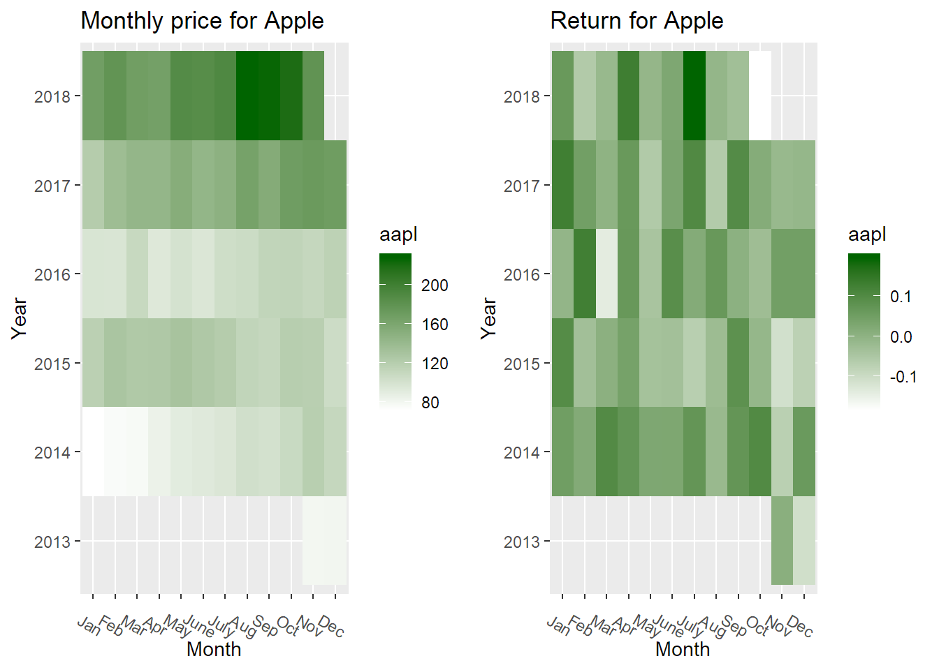 Fig 1 (a)
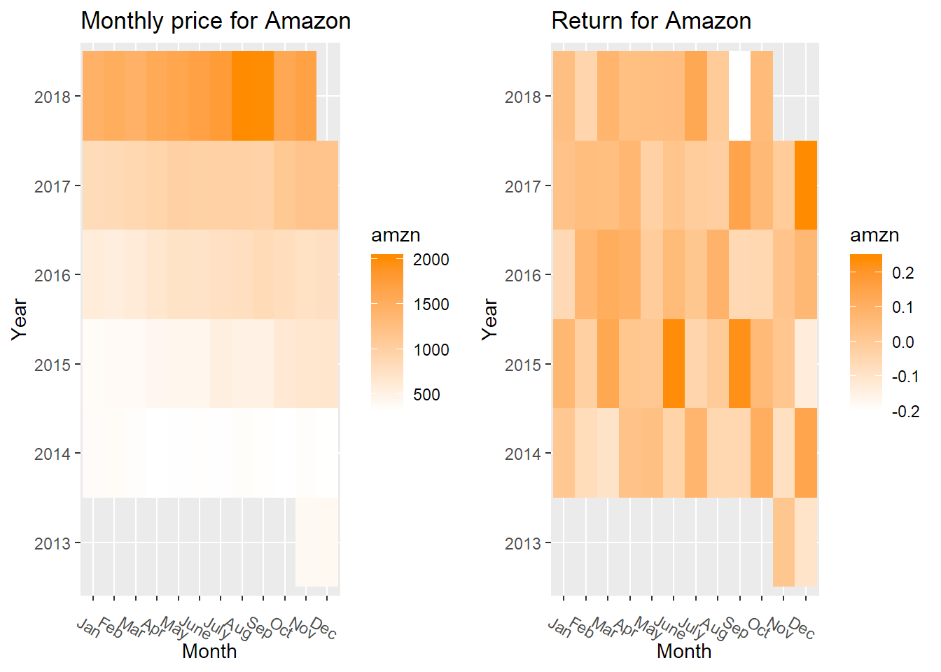 Fig 1 (b)
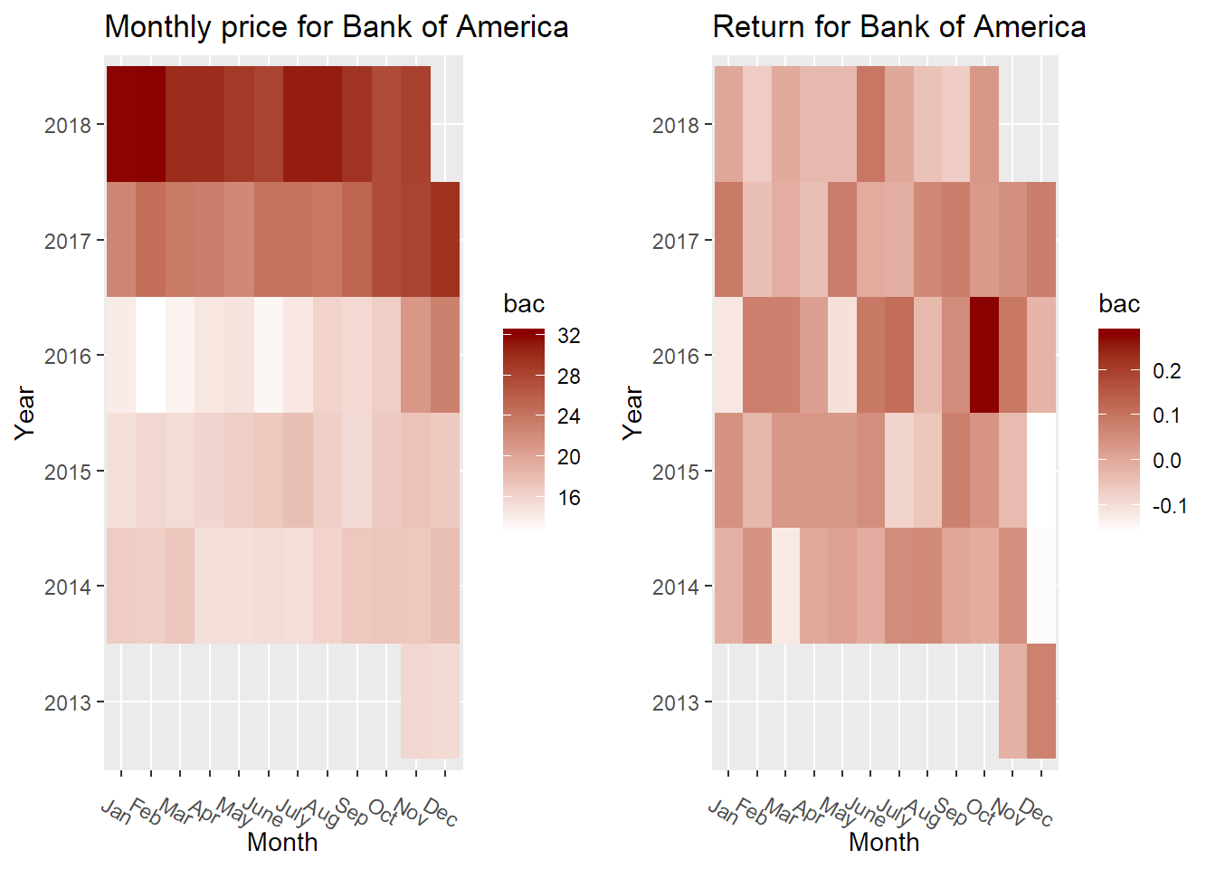 Fig 1 (c)
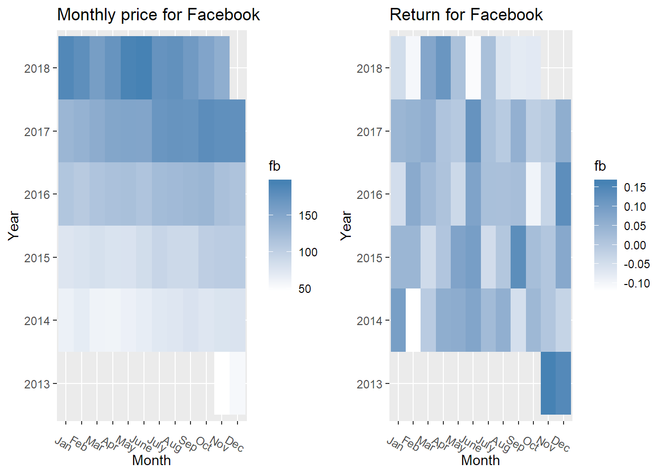 Fig 1 (d)
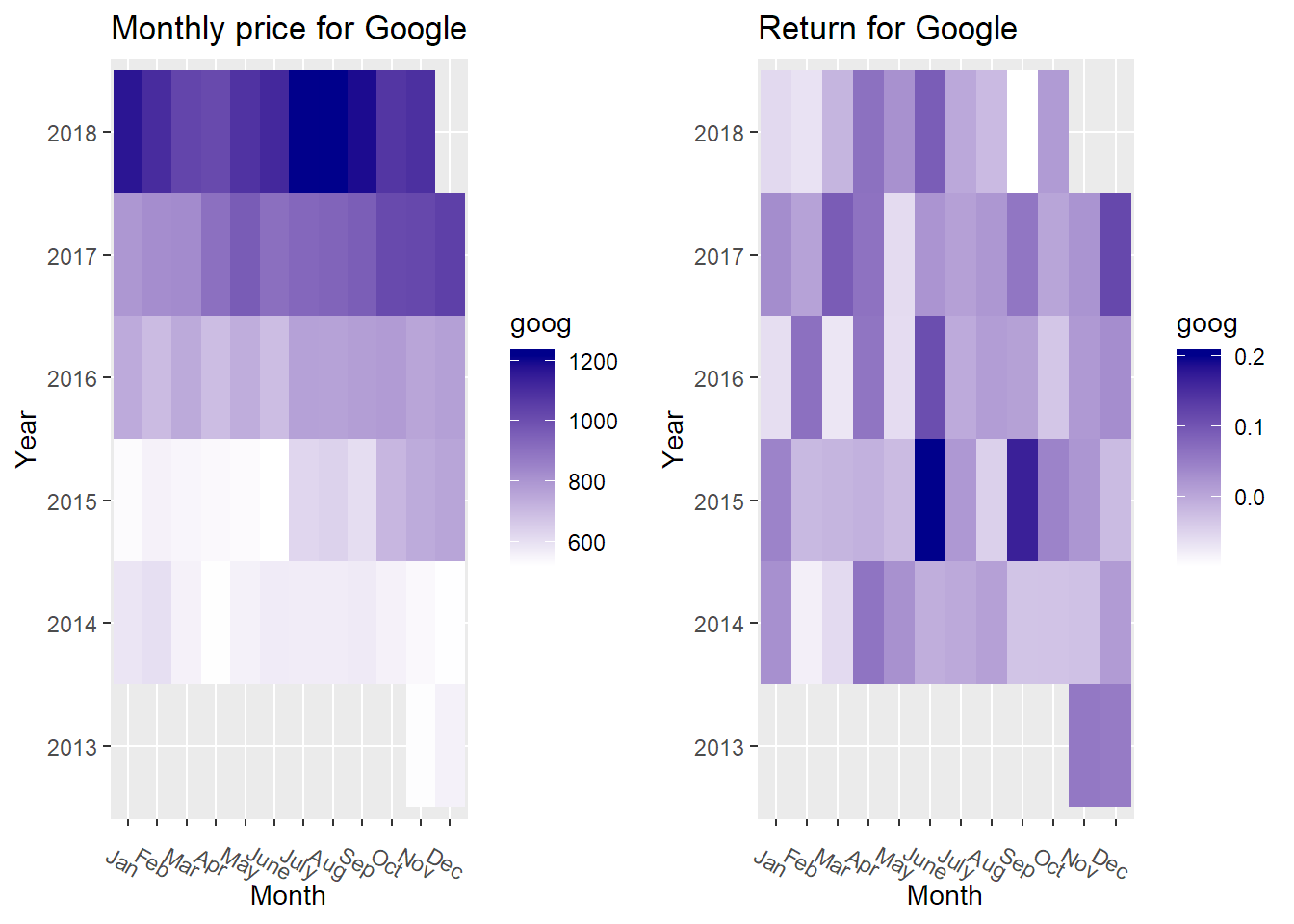 Fig 1 (e)
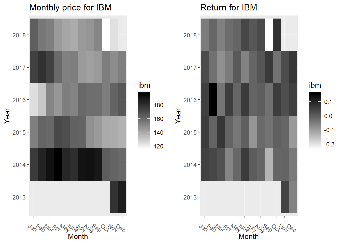 Fig 1 (f)
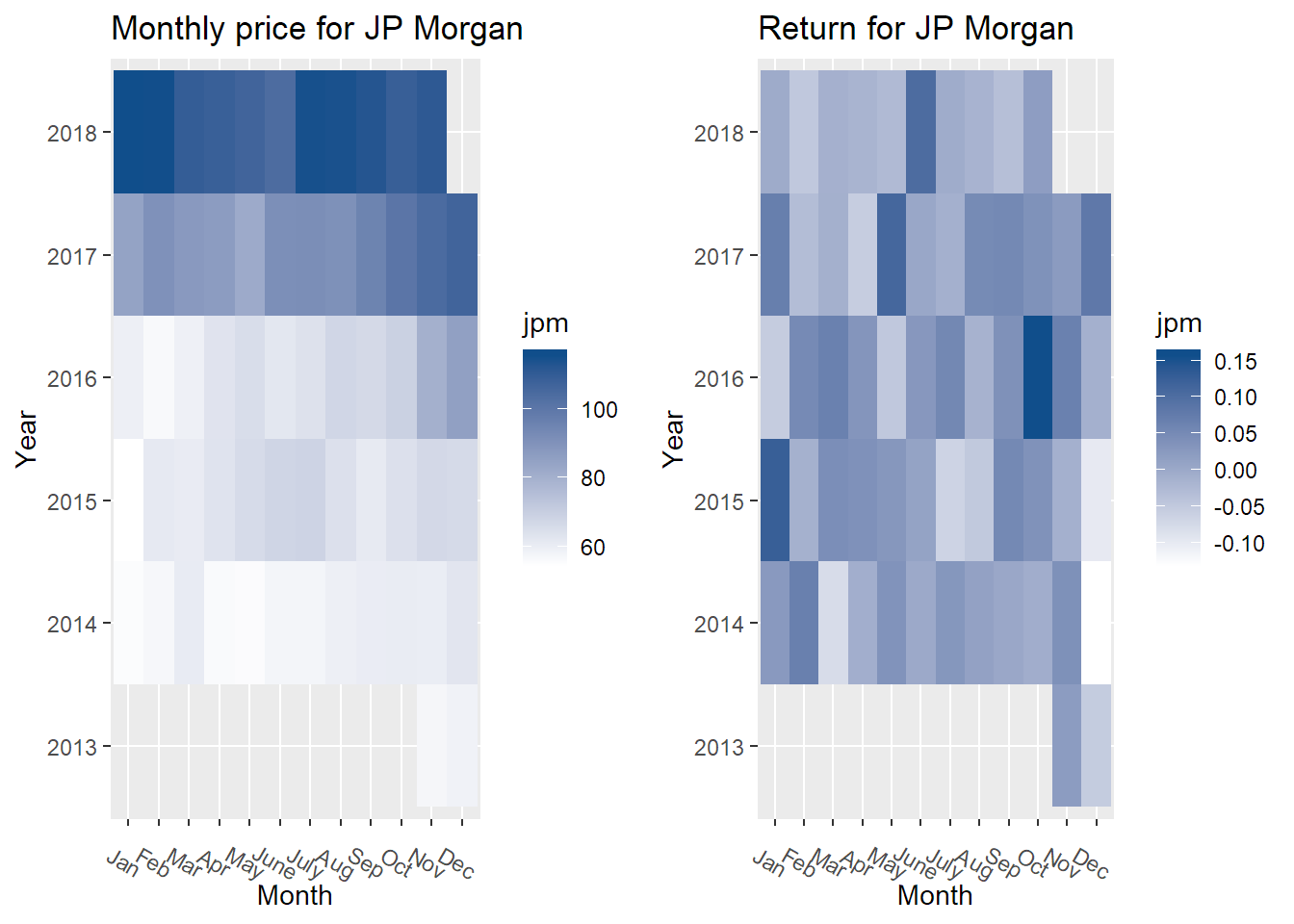 Fig 1 (g)
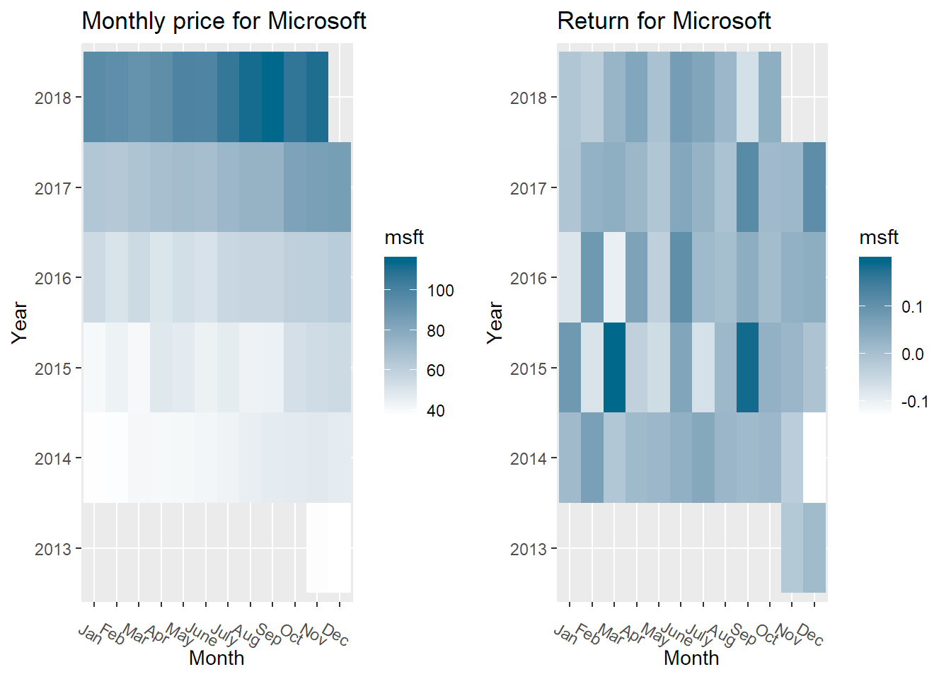 Fig 1 (h)
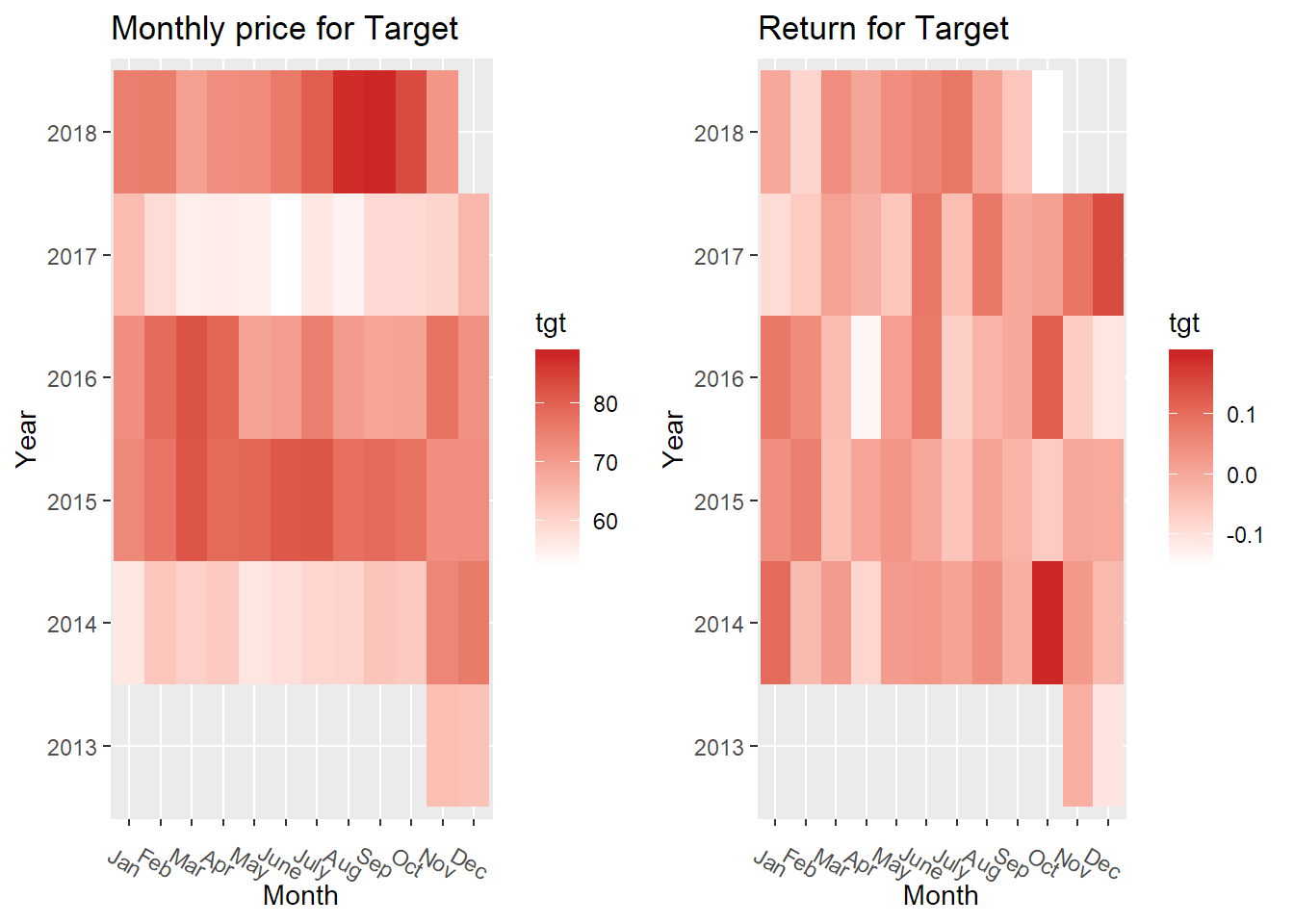 Fig 1 (i)
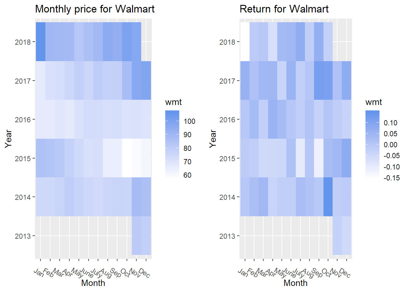 Fig 1 (j)
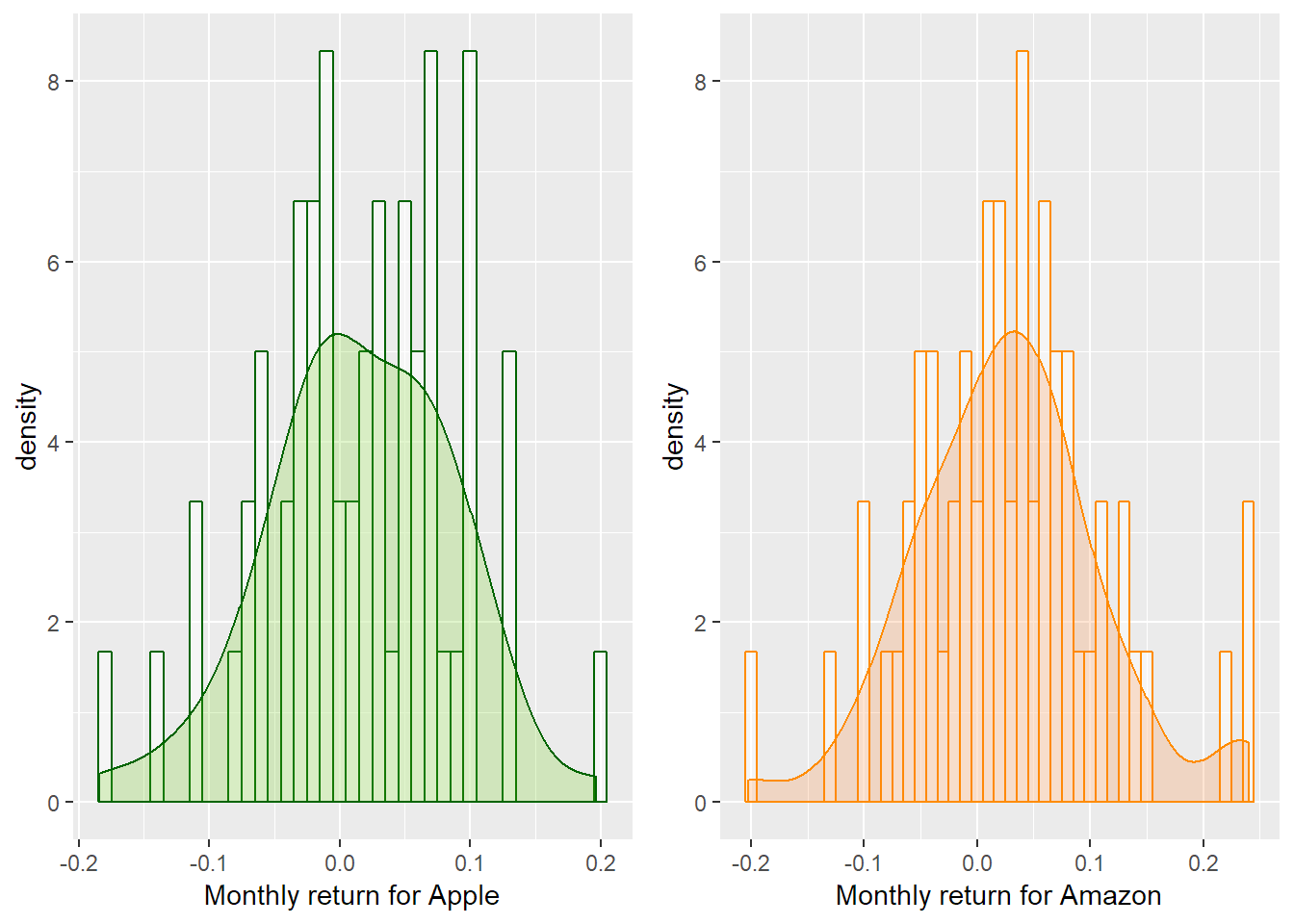 Fig 2 (a)
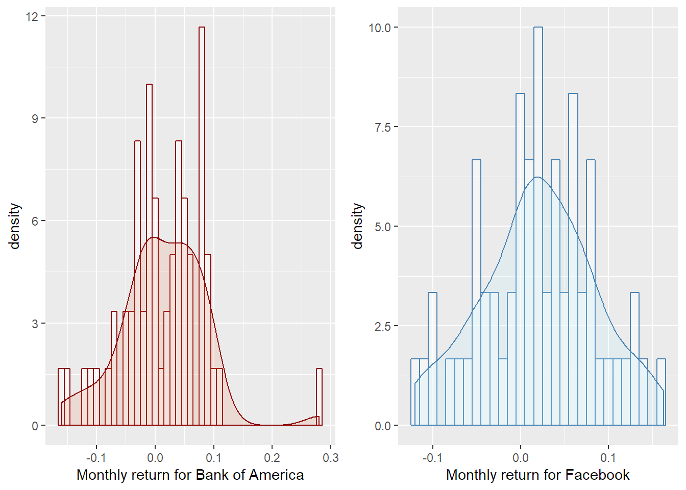 Fig 2 (b)
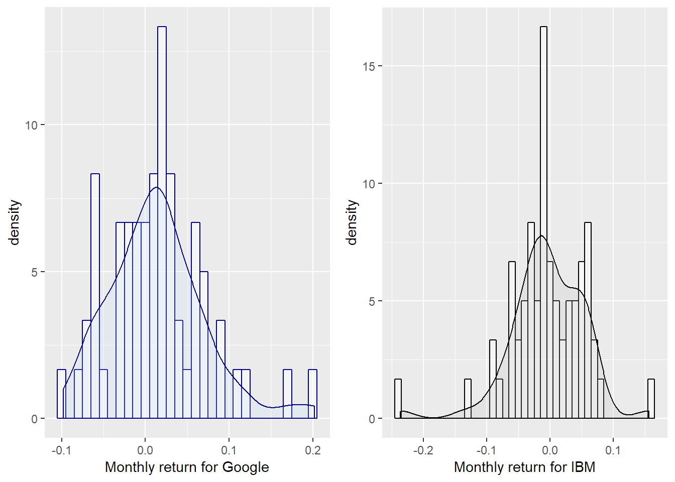 Fig 2 (c)
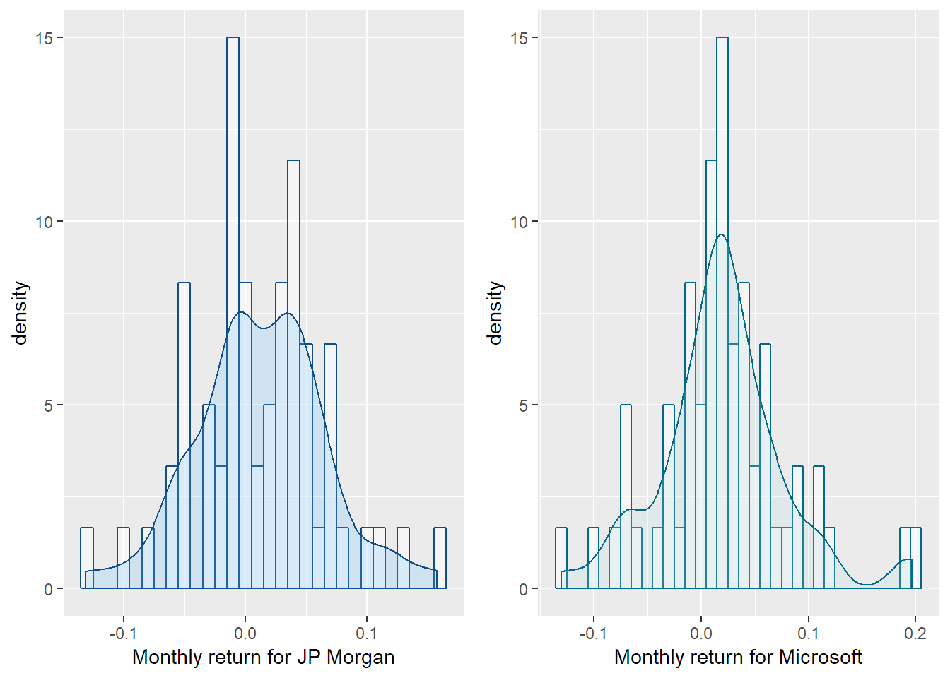 Fig 2 (d)
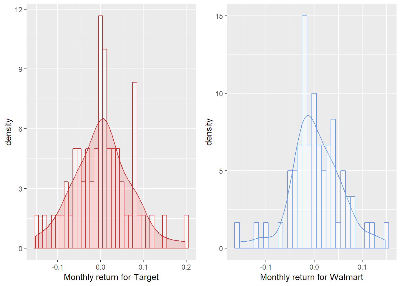 Fig 2 (e)
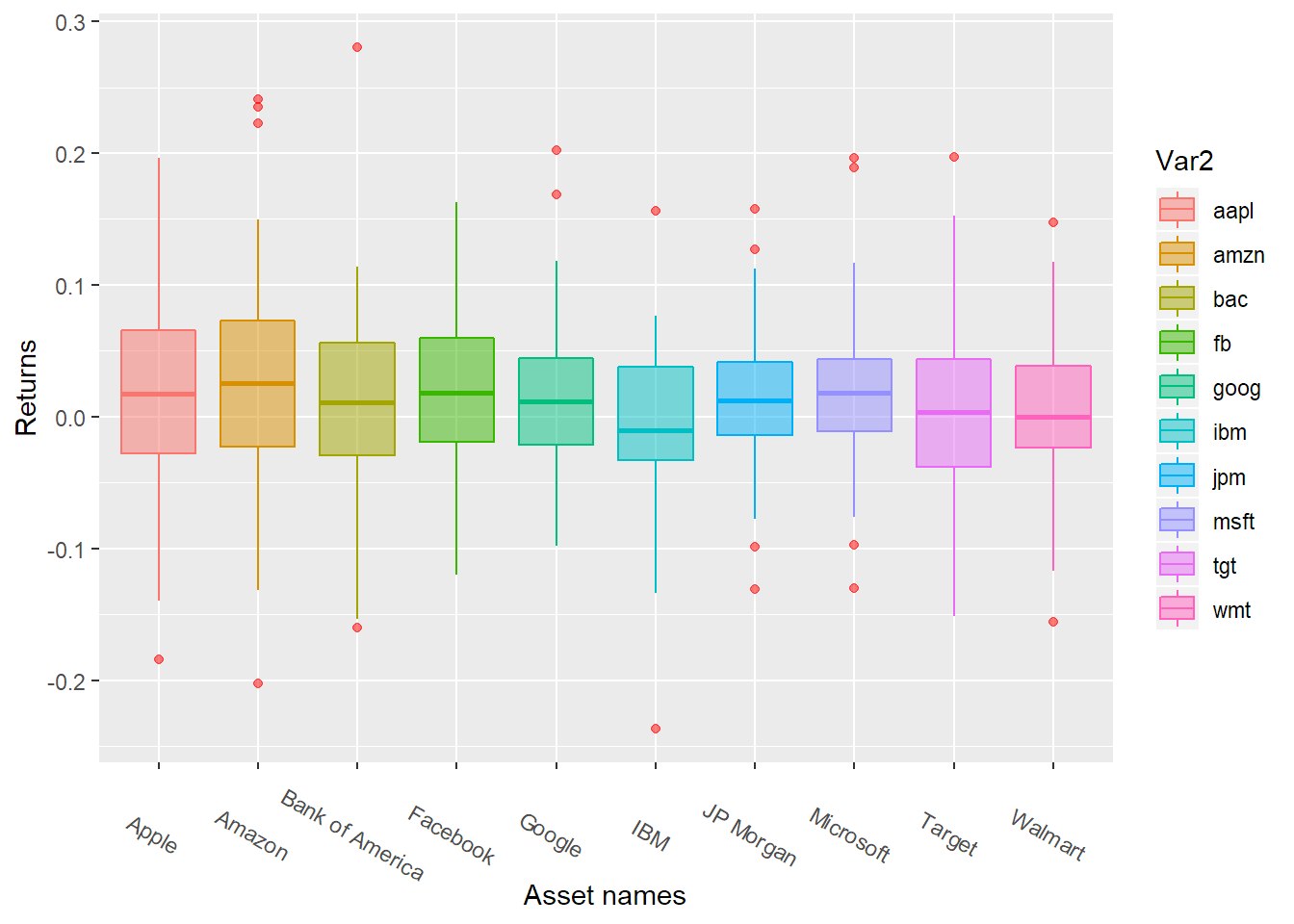 Fig 3
Fig 3
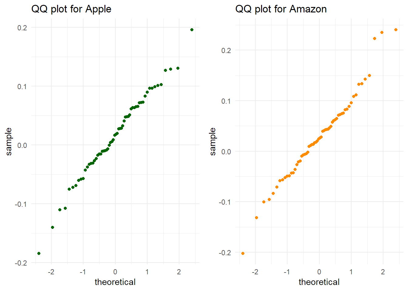 Fig 4 (a)
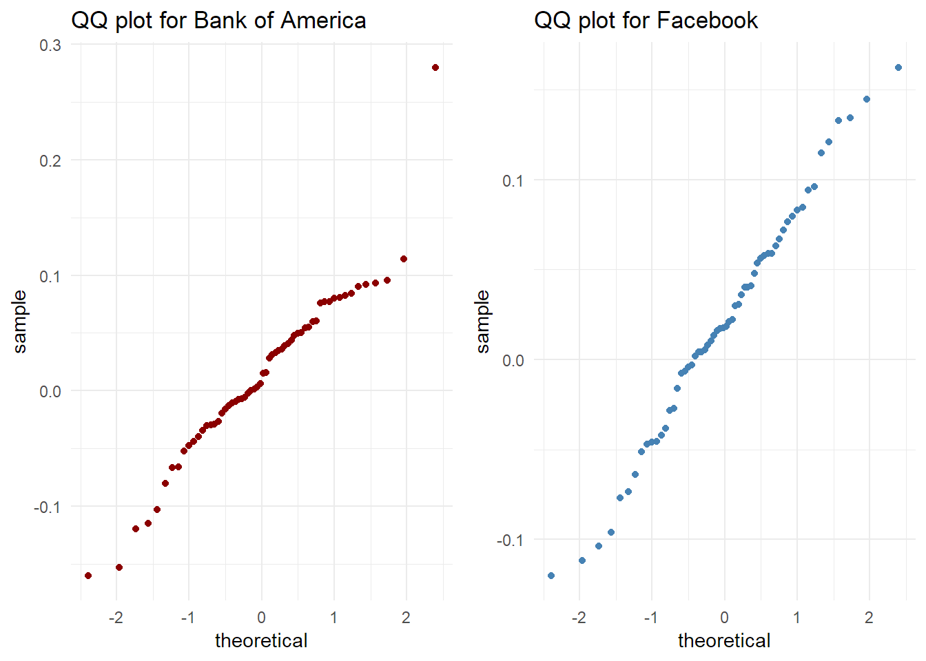 Fig 4 (b)
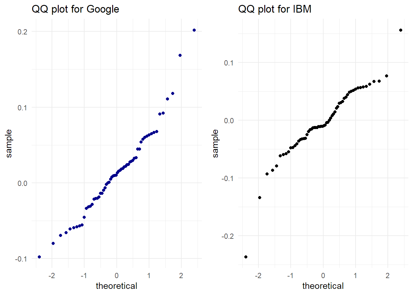 Fig 4 (c)
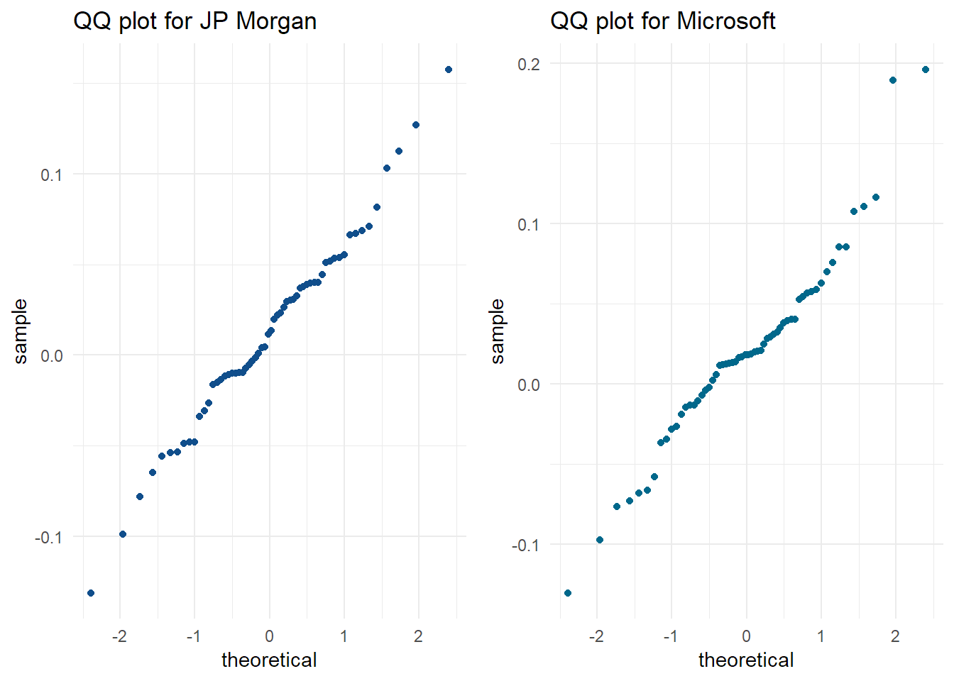 Fig 4 (d)
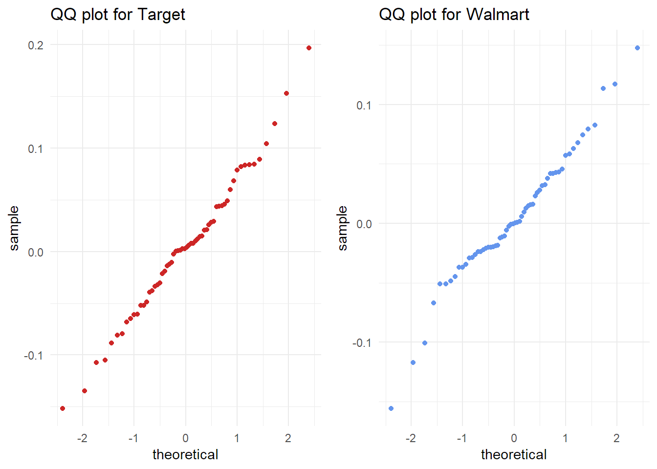 Fig 4 (e)
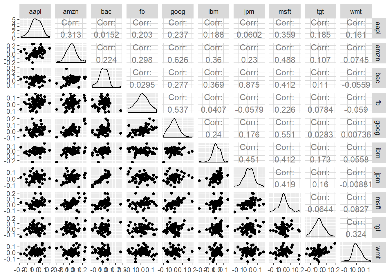 Fig 5
Fig 5
